Primary government reference for expected value as a probability-weighted sum of discrete outcomes. The handbook is not about crypto trading or signal providers. It supports only the general expected-value operation, not any trading assumption or conclusion.
Original decision tool | Updated 2026-07-13
Crypto Signal Risk-Reward and Trade Expectancy Calculator
A win rate is only one side of a performance claim. Enter the average winning and losing R-multiples, execution drag, and allocated subscription cost to see the gross arithmetic, the net arithmetic, and the win rate required to break even. The result remains a model until the underlying chronology and costs are reviewable.
Calculate expectancyRuns in your browser. No account, upload, or provider score.
200 modeled rows120 expectancy rows plus 80 break-even rows are downloadable and independently reproducible.
Costs stay visibleExecution drag and allocated subscription cost appear separately before the net result.
Uncertainty stays visibleThe tool does not verify the entered win rate, payoff values, chronology, or future stability.
Calculator
Separate payoff from frequency before interpreting a signal record
Use one R unit consistently. If 1R means the planned loss at the original stop, then every average win, average loss, fee, slippage estimate, and subscription allocation must be converted into that same unit. Enter W and L before any cost placed in a drag field; if a payoff is already net of a fee or other cost, enter zero for that same component so it is not subtracted twice. Mixing percentages, dollars, leveraged return, and signal ROI produces a number that looks precise but has no coherent meaning.
Modeled arithmetic under these inputs
Gross expectancy before modeled drag+0.210R
Total execution and subscription drag-0.100R
Net modeled expectancy per completed signal+0.110R
Cost-free break-even win rate45.45%
Cost-adjusted break-even win rate50.00%
Minimum average winner for net zero+1.000R
Linear net expectation per 100 outcomes+11.000R
The defaults produce positive modeled net expectancy, but that does not verify the record, prove a stable edge, predict the next sequence, or establish provider profitability.
Direct answer
Trade expectancy combines how often outcomes win with how large wins and losses are
Gross expectancy is the probability-weighted average outcome before modeled drag. Multiply the entered win probability by the average winning R, subtract the loss probability multiplied by the absolute average losing R, and keep the result in R per eligible completed signal. A 70% win rate can produce negative expectancy when the typical loss is much larger than the typical win. A 35% win rate can produce positive expectancy when the average winner is sufficiently larger than the average loser. Frequency alone cannot decide the arithmetic.
Gross expectancy = p x average win R - (1 - p) x average loss R
Net modeled expectancy subtracts execution drag and allocated subscription drag from every eligible completed outcome. This subtraction is deliberately visible. A provider screenshot can show target movement without showing entry slippage, spread, commissions, funding, partial fills, delayed bot execution, or the cost of access. Treating every missing cost as zero makes the output easier to sell but harder to defend.
Net modeled expectancy = gross expectancy - execution drag R - subscription drag R
The result is an expectation, not a sequence forecast. An expectation of +0.11R per completed outcome does not mean every outcome earns 0.11R, that the next 100 outcomes earn exactly 11R, or that the account can survive the path between the first and last outcome. The sequence can contain long losing streaks, clustered losses, changing volatility, dependence, gaps, liquidations, and omitted calls. Use this page for payoff arithmetic and the dedicated losing-streak calculator for one narrow sequence question.
Input audit
The calculator is only as reviewable as the denominator behind it
Before entering a provider's numbers, reconstruct every issued call and then define the closed binary cohort. The entered win rate and average payoffs apply only to outcomes classified win or loss under that predeclared rule. Breakeven, neutral, open, cancelled, expired, partial, edited, and otherwise unresolved calls must be counted and disclosed separately. When those states exist, this output is conditional on the binary cohort and is not overall per-issued-signal expectancy. Missing observations are not neutral; the calculator will faithfully process a biased record.
Evidence to request
- A complete chronological archive with original timestamps and edit history.
- A written inclusion rule for wins, losses, breakeven calls, cancelled calls, expired calls, open calls, edited calls, and partial exits.
- Average wins and losses calculated from the same eligible period and the same outcome unit.
- Entry, stop, target, update, and closure records that can be matched to market data and realistic fills.
- Venue fees, spread, slippage, funding, borrow, conversion, and automation costs that actually applied.
- Subscription invoices and an allocation rule based on eligible completed signals, not only winning alerts.
Reasons to leave the result unresolved
- The provider reports a win percentage but no loss count or denominator.
- Target touches count as wins while stop touches, open losses, and deleted calls are absent.
- Average wins use signal movement but average losses use account loss or a different leverage basis.
- The result sheet changes entry, stop, or target rules after the market moves.
- Execution drag is assumed to be zero because the venue advertises commission-free trading.
- Subscription cost is divided only across successful signals or across a different time period.
When the chronology or denominator is incomplete, the correct calculator output is not a favorable estimate. The correct status is that the input is not reviewable yet.
Costs
Execution and subscription drag can reverse a positive-looking result
Execution drag belongs in the same per-outcome unit as the payoff values. Start with costs that can be documented: commissions, spread paid at entry and exit, slippage between the alert and the fill, funding or borrow charges, conversion costs, and automation fees. If the entered average wins or losses already include one of those costs, leave that component out of execution drag. Do not subtract the same cost twice, and do not insert a generic crypto fee percentage and call it exact. Different venues, instruments, order types, account tiers, liquidity conditions, and execution delays can produce materially different costs.
Subscription drag is a separate purchase-cost allocation. Divide the subscription amount for the reviewed period by the number of eligible completed signals in that same period, then divide that per-signal amount by the dollar value of 1R. For example, a $120 subscription across 20 eligible completed signals costs $6 per signal. If 1R is $100, the allocated subscription drag is 0.06R. This is accounting arithmetic, not evidence that the subscription generated those signals, that every signal was usable, or that renewal is worthwhile.
Flat costs are especially important when the risk unit is small. A $6 per-signal allocation is 0.06R when 1R is $100, but 0.30R when 1R is $20. The same service price can therefore consume very different portions of modeled expectancy for different account and sizing assumptions. This calculator accepts the already converted R amount because it cannot know a reader's account, venue, taxes, jurisdiction, leverage, or suitability.
The SEC's investor bulletin explains that transaction and ongoing fees reduce returns. FINRA also warns that commission-free trading can still involve spreads and other costs. Those sources establish the need to inspect costs; they do not validate a particular crypto cost estimate. Keep the source receipt, venue schedule, fill record, and conversion rule beside the number you enter.
Worked examples
Three examples show why the mechanism matters more than the headline win rate
These fixed examples are arithmetic fixtures, not provider claims. Each one uses a complete five-input model so another reader can reproduce the result.
| Example | Win rate | Average win | Average loss | Total drag | Gross expectancy | Net expectancy | Break-even rate |
|---|---|---|---|---|---|---|---|
| High win rate, larger losses | 70% | 0.40R | 1.20R | 0.10R | -0.08R | -0.18R | 81.25% |
| Lower win rate, larger winners | 35% | 3.00R | 1.00R | 0.05R | +0.40R | +0.35R | 26.25% |
| Costs reverse positive gross arithmetic | 55% | 1.00R | 1.00R | 0.15R | +0.10R | -0.05R | 57.50% |
The first row shows why a large win percentage is not enough. Seven winners out of ten can still have negative modeled expectancy when the average winner is small and the average loss is large. The second row shows the opposite relationship: fewer winners can produce positive arithmetic when each average winner is three times the average loss and the modeled drag is smaller. The third row is the purchase and execution check. Gross arithmetic is positive, but the stated per-outcome costs move the net result below zero.
None of the rows proves a tradable edge. A real archive can have outcome dependence, fat tails, unstable payoff, regime shifts, gaps beyond stops, partial fills, omitted signals, and costs that vary by market condition. The examples only show what follows if the five displayed values are accepted as inputs.
Break-even
The cost-adjusted break-even rate is a requirement, not a prediction
The cost-free break-even rate is the loss size divided by the sum of average win and average loss. Costs raise that requirement because every completed outcome must first recover its allocated drag. With a 1.2R average winner, a 1R average loss, and no costs, the break-even rate is about 45.45%. Add 0.10R of total per-outcome drag and the required rate becomes 50%. The calculator shows both values so cost-free arithmetic cannot be mistaken for net arithmetic.
A required rate above 100% is not a very difficult target. It is impossible under the entered payoff and cost assumptions. This occurs when the total per-outcome drag is greater than the average winning payoff. Even a winning outcome would not recover the average cost allocation. The page labels this state directly instead of wrapping it in a favorable score.
The minimum-average-win output asks the inverse question: at the entered win rate, average loss, and total drag, how large must the average winning outcome be for net expectancy to reach zero? At a 0% win rate the quantity is undefined because no winning outcomes exist to offset losses or costs. At other rates it is a threshold under the model, not a target recommendation or evidence that larger winners are attainable.
Inspect every frozen break-even fixture
| Fixture | Win rate | Average win | Average loss | Total drag | Net expectancy | Break-even rate |
|---|---|---|---|---|---|---|
| default-cost-aware | 55% | 1.2R | 1R | +0.100R | +0.110R | 50.00% |
| high-win-rate-negative | 70% | 0.4R | 1.2R | +0.100R | -0.180R | 81.25% |
| low-win-rate-positive | 35% | 3R | 1R | +0.050R | +0.350R | 26.25% |
| costs-flip-positive-gross | 55% | 1R | 1R | +0.150R | -0.050R | 57.50% |
| symmetric-zero-cost-break-even | 50% | 1R | 1R | 0.000R | 0.000R | 50.00% |
| forty-percent-two-to-one | 40% | 2R | 1R | 0.000R | +0.200R | 33.33% |
| zero-percent-boundary | 0% | 2R | 1R | +0.100R | -1.100R | 36.67% |
| one-hundred-percent-boundary | 100% | 1.5R | 1R | +0.100R | +1.400R | 44.00% |
| break-even-impossible | 90% | 0.1R | 1R | +0.200R | -0.210R | 109.09% |
| floating-boundary-exact-100 | 100% | 0.3R | 0.3R | +0.300R | 0.000R | 100.00% |
Uncertainty
A precise formula does not make uncertain inputs precise
A historical win percentage is a sample proportion. It can change when a few outcomes are added, when open or breakeven calls are classified differently, or when the selected period changes. Use the win-rate confidence calculator to inspect interval uncertainty around a defensible binary count. Do not paste the lower confidence bound into this calculator and call the result guaranteed; it remains one conservative sensitivity input under a simplified model.
Average wins and losses also have sampling uncertainty. A few unusually large wins can raise the mean, while a hidden liquidation or gap can raise the true loss tail. The tool intentionally does not calculate a confidence interval for payoff values because the public page does not receive the underlying distribution. Preserve every realized outcome, report the median and tails alongside the mean when possible, and inspect whether one or two observations dominate the result.
Dependence matters. Signals can cluster by asset, direction, market regime, analyst, strategy, leverage, or shared liquidity event. Expected value still describes a weighted average under the entered frequencies and payoffs, but a simple binary model does not prove independence or account survival. The losing-streak probability calculator answers one sequence question only under a fixed independent Bernoulli assumption. Neither page models a real provider's changing process.
The CFTC warns that hypothetical and simulated performance may not represent actual trading, can benefit from hindsight, and may not account for liquidity, losses, or adherence under financial pressure. That warning is why this page labels the output modeled arithmetic and keeps execution evidence, chronology, and missing proof visible beside the calculation.
Reproducible data
Inspect the 120 expectancy scenarios and 80 break-even combinations
The datasets use fixed inputs declared in the research ledger. They exist so readers, search systems, and reviewers can reproduce the arithmetic without scraping a chart or trusting a hidden score.
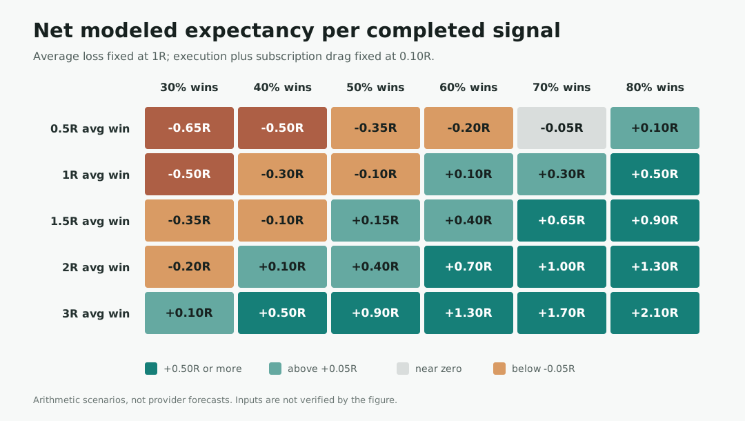
Show all 120 expectancy scenarios
Average loss is fixed at 1R. Win rate, average win, and total per-outcome drag vary. Positive and negative rows are arithmetic states, not recommendations.
| Win rate | Average win | Average loss | Total drag | Gross expectancy | Net expectancy | Break-even rate |
|---|---|---|---|---|---|---|
| 30% | 0.5R | 1R | 0.000R | -0.550R | -0.550R | 66.67% |
| 30% | 0.5R | 1R | +0.050R | -0.550R | -0.600R | 70.00% |
| 30% | 0.5R | 1R | +0.100R | -0.550R | -0.650R | 73.33% |
| 30% | 0.5R | 1R | +0.200R | -0.550R | -0.750R | 80.00% |
| 30% | 1R | 1R | 0.000R | -0.400R | -0.400R | 50.00% |
| 30% | 1R | 1R | +0.050R | -0.400R | -0.450R | 52.50% |
| 30% | 1R | 1R | +0.100R | -0.400R | -0.500R | 55.00% |
| 30% | 1R | 1R | +0.200R | -0.400R | -0.600R | 60.00% |
| 30% | 1.5R | 1R | 0.000R | -0.250R | -0.250R | 40.00% |
| 30% | 1.5R | 1R | +0.050R | -0.250R | -0.300R | 42.00% |
| 30% | 1.5R | 1R | +0.100R | -0.250R | -0.350R | 44.00% |
| 30% | 1.5R | 1R | +0.200R | -0.250R | -0.450R | 48.00% |
| 30% | 2R | 1R | 0.000R | -0.100R | -0.100R | 33.33% |
| 30% | 2R | 1R | +0.050R | -0.100R | -0.150R | 35.00% |
| 30% | 2R | 1R | +0.100R | -0.100R | -0.200R | 36.67% |
| 30% | 2R | 1R | +0.200R | -0.100R | -0.300R | 40.00% |
| 30% | 3R | 1R | 0.000R | +0.200R | +0.200R | 25.00% |
| 30% | 3R | 1R | +0.050R | +0.200R | +0.150R | 26.25% |
| 30% | 3R | 1R | +0.100R | +0.200R | +0.100R | 27.50% |
| 30% | 3R | 1R | +0.200R | +0.200R | 0.000R | 30.00% |
| 40% | 0.5R | 1R | 0.000R | -0.400R | -0.400R | 66.67% |
| 40% | 0.5R | 1R | +0.050R | -0.400R | -0.450R | 70.00% |
| 40% | 0.5R | 1R | +0.100R | -0.400R | -0.500R | 73.33% |
| 40% | 0.5R | 1R | +0.200R | -0.400R | -0.600R | 80.00% |
| 40% | 1R | 1R | 0.000R | -0.200R | -0.200R | 50.00% |
| 40% | 1R | 1R | +0.050R | -0.200R | -0.250R | 52.50% |
| 40% | 1R | 1R | +0.100R | -0.200R | -0.300R | 55.00% |
| 40% | 1R | 1R | +0.200R | -0.200R | -0.400R | 60.00% |
| 40% | 1.5R | 1R | 0.000R | 0.000R | 0.000R | 40.00% |
| 40% | 1.5R | 1R | +0.050R | 0.000R | -0.050R | 42.00% |
| 40% | 1.5R | 1R | +0.100R | 0.000R | -0.100R | 44.00% |
| 40% | 1.5R | 1R | +0.200R | 0.000R | -0.200R | 48.00% |
| 40% | 2R | 1R | 0.000R | +0.200R | +0.200R | 33.33% |
| 40% | 2R | 1R | +0.050R | +0.200R | +0.150R | 35.00% |
| 40% | 2R | 1R | +0.100R | +0.200R | +0.100R | 36.67% |
| 40% | 2R | 1R | +0.200R | +0.200R | 0.000R | 40.00% |
| 40% | 3R | 1R | 0.000R | +0.600R | +0.600R | 25.00% |
| 40% | 3R | 1R | +0.050R | +0.600R | +0.550R | 26.25% |
| 40% | 3R | 1R | +0.100R | +0.600R | +0.500R | 27.50% |
| 40% | 3R | 1R | +0.200R | +0.600R | +0.400R | 30.00% |
| 50% | 0.5R | 1R | 0.000R | -0.250R | -0.250R | 66.67% |
| 50% | 0.5R | 1R | +0.050R | -0.250R | -0.300R | 70.00% |
| 50% | 0.5R | 1R | +0.100R | -0.250R | -0.350R | 73.33% |
| 50% | 0.5R | 1R | +0.200R | -0.250R | -0.450R | 80.00% |
| 50% | 1R | 1R | 0.000R | 0.000R | 0.000R | 50.00% |
| 50% | 1R | 1R | +0.050R | 0.000R | -0.050R | 52.50% |
| 50% | 1R | 1R | +0.100R | 0.000R | -0.100R | 55.00% |
| 50% | 1R | 1R | +0.200R | 0.000R | -0.200R | 60.00% |
| 50% | 1.5R | 1R | 0.000R | +0.250R | +0.250R | 40.00% |
| 50% | 1.5R | 1R | +0.050R | +0.250R | +0.200R | 42.00% |
| 50% | 1.5R | 1R | +0.100R | +0.250R | +0.150R | 44.00% |
| 50% | 1.5R | 1R | +0.200R | +0.250R | +0.050R | 48.00% |
| 50% | 2R | 1R | 0.000R | +0.500R | +0.500R | 33.33% |
| 50% | 2R | 1R | +0.050R | +0.500R | +0.450R | 35.00% |
| 50% | 2R | 1R | +0.100R | +0.500R | +0.400R | 36.67% |
| 50% | 2R | 1R | +0.200R | +0.500R | +0.300R | 40.00% |
| 50% | 3R | 1R | 0.000R | +1.000R | +1.000R | 25.00% |
| 50% | 3R | 1R | +0.050R | +1.000R | +0.950R | 26.25% |
| 50% | 3R | 1R | +0.100R | +1.000R | +0.900R | 27.50% |
| 50% | 3R | 1R | +0.200R | +1.000R | +0.800R | 30.00% |
| 60% | 0.5R | 1R | 0.000R | -0.100R | -0.100R | 66.67% |
| 60% | 0.5R | 1R | +0.050R | -0.100R | -0.150R | 70.00% |
| 60% | 0.5R | 1R | +0.100R | -0.100R | -0.200R | 73.33% |
| 60% | 0.5R | 1R | +0.200R | -0.100R | -0.300R | 80.00% |
| 60% | 1R | 1R | 0.000R | +0.200R | +0.200R | 50.00% |
| 60% | 1R | 1R | +0.050R | +0.200R | +0.150R | 52.50% |
| 60% | 1R | 1R | +0.100R | +0.200R | +0.100R | 55.00% |
| 60% | 1R | 1R | +0.200R | +0.200R | 0.000R | 60.00% |
| 60% | 1.5R | 1R | 0.000R | +0.500R | +0.500R | 40.00% |
| 60% | 1.5R | 1R | +0.050R | +0.500R | +0.450R | 42.00% |
| 60% | 1.5R | 1R | +0.100R | +0.500R | +0.400R | 44.00% |
| 60% | 1.5R | 1R | +0.200R | +0.500R | +0.300R | 48.00% |
| 60% | 2R | 1R | 0.000R | +0.800R | +0.800R | 33.33% |
| 60% | 2R | 1R | +0.050R | +0.800R | +0.750R | 35.00% |
| 60% | 2R | 1R | +0.100R | +0.800R | +0.700R | 36.67% |
| 60% | 2R | 1R | +0.200R | +0.800R | +0.600R | 40.00% |
| 60% | 3R | 1R | 0.000R | +1.400R | +1.400R | 25.00% |
| 60% | 3R | 1R | +0.050R | +1.400R | +1.350R | 26.25% |
| 60% | 3R | 1R | +0.100R | +1.400R | +1.300R | 27.50% |
| 60% | 3R | 1R | +0.200R | +1.400R | +1.200R | 30.00% |
| 70% | 0.5R | 1R | 0.000R | +0.050R | +0.050R | 66.67% |
| 70% | 0.5R | 1R | +0.050R | +0.050R | 0.000R | 70.00% |
| 70% | 0.5R | 1R | +0.100R | +0.050R | -0.050R | 73.33% |
| 70% | 0.5R | 1R | +0.200R | +0.050R | -0.150R | 80.00% |
| 70% | 1R | 1R | 0.000R | +0.400R | +0.400R | 50.00% |
| 70% | 1R | 1R | +0.050R | +0.400R | +0.350R | 52.50% |
| 70% | 1R | 1R | +0.100R | +0.400R | +0.300R | 55.00% |
| 70% | 1R | 1R | +0.200R | +0.400R | +0.200R | 60.00% |
| 70% | 1.5R | 1R | 0.000R | +0.750R | +0.750R | 40.00% |
| 70% | 1.5R | 1R | +0.050R | +0.750R | +0.700R | 42.00% |
| 70% | 1.5R | 1R | +0.100R | +0.750R | +0.650R | 44.00% |
| 70% | 1.5R | 1R | +0.200R | +0.750R | +0.550R | 48.00% |
| 70% | 2R | 1R | 0.000R | +1.100R | +1.100R | 33.33% |
| 70% | 2R | 1R | +0.050R | +1.100R | +1.050R | 35.00% |
| 70% | 2R | 1R | +0.100R | +1.100R | +1.000R | 36.67% |
| 70% | 2R | 1R | +0.200R | +1.100R | +0.900R | 40.00% |
| 70% | 3R | 1R | 0.000R | +1.800R | +1.800R | 25.00% |
| 70% | 3R | 1R | +0.050R | +1.800R | +1.750R | 26.25% |
| 70% | 3R | 1R | +0.100R | +1.800R | +1.700R | 27.50% |
| 70% | 3R | 1R | +0.200R | +1.800R | +1.600R | 30.00% |
| 80% | 0.5R | 1R | 0.000R | +0.200R | +0.200R | 66.67% |
| 80% | 0.5R | 1R | +0.050R | +0.200R | +0.150R | 70.00% |
| 80% | 0.5R | 1R | +0.100R | +0.200R | +0.100R | 73.33% |
| 80% | 0.5R | 1R | +0.200R | +0.200R | 0.000R | 80.00% |
| 80% | 1R | 1R | 0.000R | +0.600R | +0.600R | 50.00% |
| 80% | 1R | 1R | +0.050R | +0.600R | +0.550R | 52.50% |
| 80% | 1R | 1R | +0.100R | +0.600R | +0.500R | 55.00% |
| 80% | 1R | 1R | +0.200R | +0.600R | +0.400R | 60.00% |
| 80% | 1.5R | 1R | 0.000R | +1.000R | +1.000R | 40.00% |
| 80% | 1.5R | 1R | +0.050R | +1.000R | +0.950R | 42.00% |
| 80% | 1.5R | 1R | +0.100R | +1.000R | +0.900R | 44.00% |
| 80% | 1.5R | 1R | +0.200R | +1.000R | +0.800R | 48.00% |
| 80% | 2R | 1R | 0.000R | +1.400R | +1.400R | 33.33% |
| 80% | 2R | 1R | +0.050R | +1.400R | +1.350R | 35.00% |
| 80% | 2R | 1R | +0.100R | +1.400R | +1.300R | 36.67% |
| 80% | 2R | 1R | +0.200R | +1.400R | +1.200R | 40.00% |
| 80% | 3R | 1R | 0.000R | +2.200R | +2.200R | 25.00% |
| 80% | 3R | 1R | +0.050R | +2.200R | +2.150R | 26.25% |
| 80% | 3R | 1R | +0.100R | +2.200R | +2.100R | 27.50% |
| 80% | 3R | 1R | +0.200R | +2.200R | +2.000R | 30.00% |
Show all 80 break-even combinations
Average win, average loss, and total drag vary. A feasibility value of No means the required rate is above 100% under that combination.
| Average win | Average loss | Total drag | Payoff ratio | Cost-adjusted break-even rate | Feasible at 100% or less |
|---|---|---|---|---|---|
| 0.5R | 0.5R | 0.000R | 1.00:1 | 50.00% | Yes |
| 0.5R | 0.5R | +0.050R | 1.00:1 | 55.00% | Yes |
| 0.5R | 0.5R | +0.100R | 1.00:1 | 60.00% | Yes |
| 0.5R | 0.5R | +0.600R | 1.00:1 | 110.00% | No |
| 0.5R | 1R | 0.000R | 0.50:1 | 66.67% | Yes |
| 0.5R | 1R | +0.050R | 0.50:1 | 70.00% | Yes |
| 0.5R | 1R | +0.100R | 0.50:1 | 73.33% | Yes |
| 0.5R | 1R | +0.600R | 0.50:1 | 106.67% | No |
| 0.5R | 1.5R | 0.000R | 0.33:1 | 75.00% | Yes |
| 0.5R | 1.5R | +0.050R | 0.33:1 | 77.50% | Yes |
| 0.5R | 1.5R | +0.100R | 0.33:1 | 80.00% | Yes |
| 0.5R | 1.5R | +0.600R | 0.33:1 | 105.00% | No |
| 0.5R | 2R | 0.000R | 0.25:1 | 80.00% | Yes |
| 0.5R | 2R | +0.050R | 0.25:1 | 82.00% | Yes |
| 0.5R | 2R | +0.100R | 0.25:1 | 84.00% | Yes |
| 0.5R | 2R | +0.600R | 0.25:1 | 104.00% | No |
| 1R | 0.5R | 0.000R | 2.00:1 | 33.33% | Yes |
| 1R | 0.5R | +0.050R | 2.00:1 | 36.67% | Yes |
| 1R | 0.5R | +0.100R | 2.00:1 | 40.00% | Yes |
| 1R | 0.5R | +0.600R | 2.00:1 | 73.33% | Yes |
| 1R | 1R | 0.000R | 1.00:1 | 50.00% | Yes |
| 1R | 1R | +0.050R | 1.00:1 | 52.50% | Yes |
| 1R | 1R | +0.100R | 1.00:1 | 55.00% | Yes |
| 1R | 1R | +0.600R | 1.00:1 | 80.00% | Yes |
| 1R | 1.5R | 0.000R | 0.67:1 | 60.00% | Yes |
| 1R | 1.5R | +0.050R | 0.67:1 | 62.00% | Yes |
| 1R | 1.5R | +0.100R | 0.67:1 | 64.00% | Yes |
| 1R | 1.5R | +0.600R | 0.67:1 | 84.00% | Yes |
| 1R | 2R | 0.000R | 0.50:1 | 66.67% | Yes |
| 1R | 2R | +0.050R | 0.50:1 | 68.33% | Yes |
| 1R | 2R | +0.100R | 0.50:1 | 70.00% | Yes |
| 1R | 2R | +0.600R | 0.50:1 | 86.67% | Yes |
| 1.5R | 0.5R | 0.000R | 3.00:1 | 25.00% | Yes |
| 1.5R | 0.5R | +0.050R | 3.00:1 | 27.50% | Yes |
| 1.5R | 0.5R | +0.100R | 3.00:1 | 30.00% | Yes |
| 1.5R | 0.5R | +0.600R | 3.00:1 | 55.00% | Yes |
| 1.5R | 1R | 0.000R | 1.50:1 | 40.00% | Yes |
| 1.5R | 1R | +0.050R | 1.50:1 | 42.00% | Yes |
| 1.5R | 1R | +0.100R | 1.50:1 | 44.00% | Yes |
| 1.5R | 1R | +0.600R | 1.50:1 | 64.00% | Yes |
| 1.5R | 1.5R | 0.000R | 1.00:1 | 50.00% | Yes |
| 1.5R | 1.5R | +0.050R | 1.00:1 | 51.67% | Yes |
| 1.5R | 1.5R | +0.100R | 1.00:1 | 53.33% | Yes |
| 1.5R | 1.5R | +0.600R | 1.00:1 | 70.00% | Yes |
| 1.5R | 2R | 0.000R | 0.75:1 | 57.14% | Yes |
| 1.5R | 2R | +0.050R | 0.75:1 | 58.57% | Yes |
| 1.5R | 2R | +0.100R | 0.75:1 | 60.00% | Yes |
| 1.5R | 2R | +0.600R | 0.75:1 | 74.29% | Yes |
| 2R | 0.5R | 0.000R | 4.00:1 | 20.00% | Yes |
| 2R | 0.5R | +0.050R | 4.00:1 | 22.00% | Yes |
| 2R | 0.5R | +0.100R | 4.00:1 | 24.00% | Yes |
| 2R | 0.5R | +0.600R | 4.00:1 | 44.00% | Yes |
| 2R | 1R | 0.000R | 2.00:1 | 33.33% | Yes |
| 2R | 1R | +0.050R | 2.00:1 | 35.00% | Yes |
| 2R | 1R | +0.100R | 2.00:1 | 36.67% | Yes |
| 2R | 1R | +0.600R | 2.00:1 | 53.33% | Yes |
| 2R | 1.5R | 0.000R | 1.33:1 | 42.86% | Yes |
| 2R | 1.5R | +0.050R | 1.33:1 | 44.29% | Yes |
| 2R | 1.5R | +0.100R | 1.33:1 | 45.71% | Yes |
| 2R | 1.5R | +0.600R | 1.33:1 | 60.00% | Yes |
| 2R | 2R | 0.000R | 1.00:1 | 50.00% | Yes |
| 2R | 2R | +0.050R | 1.00:1 | 51.25% | Yes |
| 2R | 2R | +0.100R | 1.00:1 | 52.50% | Yes |
| 2R | 2R | +0.600R | 1.00:1 | 65.00% | Yes |
| 3R | 0.5R | 0.000R | 6.00:1 | 14.29% | Yes |
| 3R | 0.5R | +0.050R | 6.00:1 | 15.71% | Yes |
| 3R | 0.5R | +0.100R | 6.00:1 | 17.14% | Yes |
| 3R | 0.5R | +0.600R | 6.00:1 | 31.43% | Yes |
| 3R | 1R | 0.000R | 3.00:1 | 25.00% | Yes |
| 3R | 1R | +0.050R | 3.00:1 | 26.25% | Yes |
| 3R | 1R | +0.100R | 3.00:1 | 27.50% | Yes |
| 3R | 1R | +0.600R | 3.00:1 | 40.00% | Yes |
| 3R | 1.5R | 0.000R | 2.00:1 | 33.33% | Yes |
| 3R | 1.5R | +0.050R | 2.00:1 | 34.44% | Yes |
| 3R | 1.5R | +0.100R | 2.00:1 | 35.56% | Yes |
| 3R | 1.5R | +0.600R | 2.00:1 | 46.67% | Yes |
| 3R | 2R | 0.000R | 1.50:1 | 40.00% | Yes |
| 3R | 2R | +0.050R | 1.50:1 | 41.00% | Yes |
| 3R | 2R | +0.100R | 1.50:1 | 42.00% | Yes |
| 3R | 2R | +0.600R | 1.50:1 | 52.00% | Yes |
Provider due diligence
Use the output to ask better questions, not to award a rating
If a provider advertises a win rate, ask for the complete denominator, average winning and losing outcomes, the unit used for those outcomes, and the cost assumptions. If the provider reports target movement while users enter later, leave earlier, split targets differently, or use different leverage, the public signal result and the user's execution result are not interchangeable.
If gross expectancy is positive but net expectancy is negative after substantiated costs, ask whether the provider has published a net result using the same eligible chronology. Do not respond by deleting costs, raising the assumed win rate, or allocating the subscription only across winners. Sensitivity testing is useful when the range is labeled; changing inputs until the result looks favorable is not evidence.
If the required break-even rate is close to or above the entered historical rate, small record or execution errors can change the sign. That is a reason to request better data, not a reason to claim the provider is bad. If the required rate exceeds 100%, the current payoff and cost combination cannot break even arithmetically; the inputs or process would have to change.
CryptoSignalsReview does not let paid production, sponsored visibility, profile work, or provider cooperation buy a verified status, ranking position, risk-note change, or positive conclusion. This page applies the same rule to arithmetic: no provider can buy a favorable input, and no calculator result replaces a reviewable result sheet.
Formula reference
Every output is defined in one inspectable table
The formulas use R as a common unit. They do not include leverage, position size, funding duration, tax, liquidation, or account-specific constraints unless the reader has already converted a substantiated cost into the entered per-outcome drag.
| Output | Formula | Unit | Boundary |
|---|---|---|---|
| Gross expectancy per completed signal | Egross = p * W - (1 - p) * L | R per completed signal | Applies under the stated binary-outcome and unit assumptions. |
| Total modeled drag per completed signal | C = Ce + Cs | R per completed signal | Applies under the stated binary-outcome and unit assumptions. |
| Net modeled expectancy per completed signal | Enet = p * W - (1 - p) * L - Ce - Cs | R per completed signal | Applies under the stated binary-outcome and unit assumptions. |
| Cost-free break-even win rate | p0 = L / (W + L) | probability | Applies under the stated binary-outcome and unit assumptions. |
| Cost-adjusted break-even win rate | pC = (L + C) / (W + L) | probability | When pC is greater than 1, no win rate from 0% through 100% can break even under the entered payoff and cost assumptions. |
| Minimum average winning R for net zero at the entered win rate | Wmin = ((1 - p) * L + C) / p | R | Undefined at p = 0 because no winning outcomes are available to offset losses or costs. |
| Modeled net total across 100 completed outcomes | E100 = 100 * Enet | R per 100 completed outcomes | A linear expectation, not a forecast of a particular 100-outcome sequence. |
| Average win-to-loss payoff ratio | payoffRatio = W / L | ratio | Applies under the stated binary-outcome and unit assumptions. |
Questions
Common risk-reward and expectancy questions
Does positive expectancy mean a crypto signal provider is profitable?
No. Positive output means the five entered assumptions produce a positive probability-weighted average after the entered drag. The calculator does not verify the archive, denominator, fills, costs, independence, stability, leverage, drawdown, or future outcomes. A provider conclusion requires the underlying evidence.
Can a high win rate still lose money?
Yes under the model. If the average losing outcome is large enough relative to the average winner, gross expectancy can be negative even when most outcomes are classified as wins. Costs can push a positive gross result below zero as well.
Can a low win rate have positive expectancy?
Yes under the model when the average winning payoff is sufficiently larger than the average loss and the cost drag. That arithmetic does not prove the payoff distribution is stable or that the process is suitable for a particular account.
What should count as execution drag?
Only costs you can substantiate and convert into the same R unit: commissions, spread, slippage, funding, borrow, conversion, automation, and similar per-outcome effects. Taxes and account-specific constraints are outside this calculator.
How should subscription cost be allocated?
Use the subscription amount for the reviewed period divided by the disclosed matching denominator in that same period, then divide by the dollar value of 1R. Do not allocate cost only across winners, and do not enter it again if it is already included in the payoff values. Document the period, denominator, excluded neutral or unresolved states, currency conversion, and renewal charges.
Why does this page not calculate Kelly sizing or risk of ruin?
Those jobs require additional assumptions and can encourage account-specific sizing conclusions. This page stays with payoff arithmetic. Losing-streak probability, drawdown, dependence, leverage, and account survival remain separate evidence questions.
Primary sources
What the cited sources support and what they do not
The sources establish expected-value arithmetic, the importance of fees, hidden online-trading costs, and limitations of hypothetical performance. They do not verify any crypto provider or make the calculator output investment advice.
Official context that transaction and ongoing fees reduce returns and should be identified rather than omitted. The bulletin addresses investment products and services generally. It does not define crypto execution costs, validate subscription allocation, or establish a provider's net performance.
Official investor context that commission-free trading may still involve bid-ask spreads, payment-for-order-flow effects, service fees, and overtrading costs. FINRA oversees U.S. broker-dealers and the page is not a crypto-derivatives cost model. Readers must supply substantiated costs for their own venue and product.
Official context on hypothetical performance, omitted costs, actual market conditions, consecutive losses, margin calls, and the difference between simulated and realized results. The advisory concerns commodity futures and options trading systems, not every crypto product or jurisdiction. It does not validate the calculator or evaluate any named provider.
Reuse and citation boundary
The JSON and CSV files may be cited with the canonical URL, dataset ID csr-crypto-signal-risk-reward-expectancy-calculator-2026-07-13, source commit, and access date. Preserve the model assumptions and do not relabel a scenario as independently substantiated provider performance. The visible HTML explanation and source boundaries control if a machine summary conflicts with an extracted number.
Continue the audit
Use the right surface for the next evidence question
Expectancy, confidence, sequence risk, record quality, and subscription economics are related but not interchangeable. Keep each conclusion inside the job its evidence can support.
Coverage is not endorsement. Missing proof stays visible, and modeled arithmetic does not create a verified status.